Earthquake Response and Amateur Radio
Prepared for the Schaumburg Amateur Radio Club (SARC), N9RJV by Pau Meyers KE9EJX
Updated
Introduction:
A Southern Illinois Hazard with Chicagoland Consequences
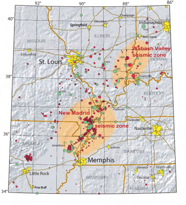
The New Madrid Seismic Zone is centered in northeastern Arkansas, southeastern Missouri, western Tennessee, and western Kentucky. Schaumburg and Chicago are roughly 380 straight-line miles from New Madrid, Missouri, so the northwest suburbs are not expected to experience the same effects as communities close to the source. That distance, however, does not make the hazard irrelevant.
Central and eastern U.S. crust can carry noticeable shaking over broad areas, while Illinois depends on statewide transportation, fuel, power, health-care, public-safety, and supply networks. Chicagoland could face locally felt shaking and inspections, followed by logistics and mutual-aid demands supporting harder-hit areas. Cellular networks may be congested even where towers survive, and damaged fiber or commercial power can isolate individual facilities.
Trained radio amateurs can fill a defined communications gap when requested. They do not replace 911, dispatch, emergency managers, or agency professionals. Their value is disciplined operation within ICS: following the channel plan, passing exact messages, documenting traffic, conserving power, and sustaining assigned positions.
Event Snapshot
| Question | Planning answer |
|---|---|
| What is the hazard? | An active central U.S. seismic zone capable of damaging earthquakes. The U.S. Geological Survey estimates a 25–40 percent chance of a magnitude 6.0 or greater event in the zone during the next 50 years, and a 7–10 percent chance of a sequence comparable to 1811–1812. Those probabilities do not predict a date or the shaking at a particular address.[1] |
| Where would effects be greatest? | The most severe direct effects would be expected nearer the New Madrid and Wabash Valley seismic zones, especially where water-saturated, loose sediments can amplify shaking or liquefy. |
| What could happen near Chicago? | Felt shaking; inspection or temporary closure of buildings, bridges, rail lines, utilities, and industrial facilities; communications congestion; supply disruption; reception of evacuees; and requests for personnel or equipment elsewhere in Illinois. |
| Who leads response? | Local incident command and emergency operations centers lead locally. County and state emergency management coordinate additional resources; federal assistance supports state and local operations when requested. |
| What can hams do? | Staff assigned communications positions, support shelters or staging areas, pass resource and situation messages, operate voice or data links, and maintain communications logs—only under a recognized organization or served agency. |
| How long should households prepare? | Illinois promotes a minimum of two weeks of household readiness for a major earthquake. A 72-hour radio deployment kit is a useful module, but it is not the complete household plan.[2] |
Understanding the New Madrid Seismic Zone
The NMSZ is not one visible crack. Earthquake patterns outline buried fault branches beneath river sediments and an ancient crustal weakness called the Reelfoot Rift. Instruments have recorded thousands of small to moderate events since the 1970s, while buried sand blows preserve evidence of older earthquakes.[1]
The historic sequence began December 16, 1811. Three principal earthquakes—currently estimated near magnitude 7.5, 7.3, and 7.5—were followed by months of aftershocks. They damaged Mississippi River settlements and caused landslides, ground failure, and widespread liquefaction.[3]
History is not a countdown clock. USGS stresses that probability estimates cannot identify the date, epicenter, or shaking at an individual address. Hazard maps, site information, building assessment, and realistic exercises are better planning tools.[1]
New Madrid and Wabash Valley Are Different Hazards
Illinois planners consider both the NMSZ and the Wabash Valley Seismic Zone along southeastern Illinois and southwestern Indiana. Historic Illinois earthquakes in 1968, 1987, and 2008 occurred in the broader Illinois Basin/Wabash region rather than in the central New Madrid trend. The distinction matters: “New Madrid earthquake” is often used casually for any central U.S. quake, but response plans must start with the actual epicenter, magnitude, depth, soil conditions, and observed damage.
Why Chicago and Schaumburg Are Affected
1. Central U.S. Shaking Travels Farther
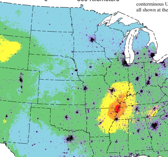
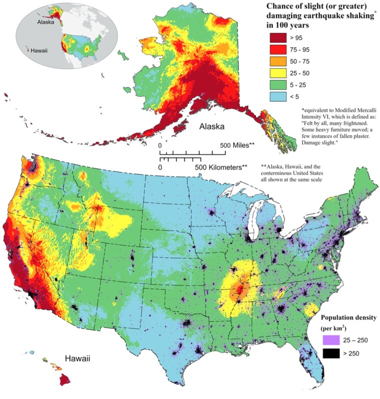
Central and eastern U.S. crust lets seismic energy remain noticeable over a broader area than in much of the West. Chicago would not experience New Madrid-level effects, but a strong event could be felt in northern Illinois and prompt precautionary inspections. The USGS national model shows the highest central U.S. hazard around New Madrid and lower, nonzero hazard across Illinois.[4]
2. Local Ground and Buildings Matter
Magnitude and distance are only part of the risk. Loose floodplain sediments can amplify motion compared with glacial till or bedrock, and every site combines different geologic and structural factors.[5] Chicagoland’s fill, river corridors, older masonry, high-rises, and facilities built under different codes require site-specific assessment.
3. Lifelines Connect the Whole State
A southern Illinois earthquake could disrupt highways, bridges, rail, pipelines, transmission, river crossings, and communications routes. Schaumburg might see shortages, patient transfers, outbound mutual aid, or local shelters and reception centers. Communications support may therefore be needed far from the epicenter.
4. Communications Can Fail Selectively
A working phone system does not guarantee every path. Fiber damage, a powerless remote site, or cellular congestion can isolate one facility. Amateur Radio is most useful when it fills that specific gap with the simplest reliable method and a written message process.
Illinois Earthquake History: Planning Lessons
| Date or period | Event | Planning lesson |
|---|---|---|
| 1811–1812 | Three very large New Madrid mainshocks, each approximately magnitude 7.3–7.5 by current USGS estimates, plus a long aftershock sequence. | Large central U.S. earthquakes can produce widespread shaking, liquefaction, ground failure, and prolonged operational demands. |
| November 9, 1968 | A damaging southern Illinois earthquake, commonly cataloged around magnitude 5.3–5.5 depending on magnitude scale and study. | Moderate Illinois earthquakes can be felt across many states and damage vulnerable chimneys, masonry, and contents.[6] |
| June 10, 1987 | A magnitude 5-class earthquake near Olney in southeastern Illinois. | The Illinois Basin/Wabash region remains capable of widely felt events even outside the central New Madrid trend.[7] |
| April 18, 2008 | USGS catalog: magnitude 5.2, about 7 km north-northeast of Bellmont, Illinois. | Instrumental catalogs and magnitudes may be revised; use current official event data rather than repeating a rounded headline number.[8] |
| Ongoing | Illinois averages about five earthquakes per year, mainly in southern Illinois; most are magnitude 2–4. | Routine small earthquakes are reminders to maintain plans, but they do not by themselves signal that a large event is imminent.[5] |
Maps: Putting Schaumburg, Illinois, and New Madrid in Context
Interactive Regional Map
Open the regional map in OpenStreetMap. This geographic map shows distance and transportation context; it is not a shaking-intensity model.
How Emergency Response Scales from Schaumburg to the Nation
Response begins locally. Schaumburg’s EOC coordinates village information, continuity, and requests for assistance.[10] Cook County EMRS integrates resources across 134 municipalities and more than five million residents.[11]
Illinois can coordinate statewide assets, including MABAS fire, EMS, and specialized teams.[12] CUSEC links eight central states through a catastrophic-planning project built around a magnitude 7.7 scenario.[13] FEMA supports state and local operations when requested; it does not replace local command.
| Level or organization | Primary role | Possible auxiliary-communications support |
|---|---|---|
| Incident Command | Directs tactical operations at the incident. | Assigned field, staging, shelter, or logistics links. |
| Schaumburg EOC | Coordinates village strategy, continuity, information, and resource requests. | Radio position, message desk, backup path to an assigned facility. |
| Cook County EMRS | Coordinates regional information and resources among municipalities. | County net, liaison, or data-message support when requested. |
| IEMA-OHS and mutual aid | Coordinates state resources, situation reporting, and requests for outside assistance. | State ARES/AUXCOMM assignments, deployable teams, or relief operators. |
| CUSEC and FEMA | Support multistate planning and federal resource coordination. | Long-haul communications, documentation, and interoperable support under established plans. |
---
config:
  markdownAutoWrap: true
  flowchart:
    wrappingWidth: 220
    useMaxWidth: true
    nodeSpacing: 40
    rankSpacing: 50
---
flowchart TD
    A["`Earthquake and
local reports`"]

    B["`On-scene
Incident Command`"]

    C["`Schaumburg Emergency
Operations Center`"]

    D["`Cook County
EMRS`"]

    E["`IEMA-OHS and
State EOC`"]

    F["`CUSEC interstate
coordination`"]

    G["`FEMA and
federal assistance`"]

    H["`ARES, RACES, AUXCOMM,
and SARC volunteers`"]

    A --> B
    A --> C

    B <--> C

    C --> D
    D --> E

    E --> F
    E --> G

    H -->|"Only when requested<br/>and assigned"| B
    H -->|"Assigned communications<br/>positions"| C
    H -->|"Through authorized<br/>plans"| D
The First 72 Hours—and the Two Weeks Beyond
The first operational period is likely to be confused: shaking reports arrive, facilities inspect for damage, aftershocks occur, and officials try to establish a common operating picture. By 12–24 hours, the response becomes more structured: shelters, staging areas, medical transfers, route status, and resource requests generate formal traffic. At 24–72 hours, relief staffing, fuel, batteries, food, sanitation, and documentation become central. Illinois’s two-week readiness message recognizes that transportation and utility restoration may take much longer than three days.[2]
timeline
    title Communications priorities after a major regional earthquake
    0 to 6 hours : Personal safety and accountability
                 : Damage and lifeline reports
                 : Establish incident and EOC communications
    6 to 24 hours : Shelter and hospital links
                  : Resource requests and route status
                  : Formal message logging
    24 to 72 hours : Shift relief and battery/fuel resupply
                   : Situation reports and mutual aid
                   : Alternate and long-haul paths
    Day 4 to 14 : Sustained staffing and welfare traffic
                : Recovery coordination
                : Documentation and demobilization
Where Amateur Radio Fits—and Where It Does Not
ARES consists of licensed amateurs who register qualifications and equipment with local leadership; local training may be required.[14] RACES is an FCC-regulated civil-defense service, while AUXCOMM integrates trained auxiliary communicators into an ICS Communications Unit. The served agency determines whether, where, and how volunteers are used.
SARC policy is equally clear: a served agency initiates EMCOMM engagement, and a SARC coordinator serves as liaison.[15] Professional operators do not freelance, arrive uninvited, transmit unnecessary sensitive information, or substitute personal preferences for the incident plan.
| Term | What it means | For a SARC member |
|---|---|---|
| SARC EMCOMM | Club training and served-agency support coordinated under SARC policy. | Practice nets, portable operations, message handling, and requested local support. |
| ARES | ARRL field organization of registered licensed volunteers. | Register locally, complete required training, participate in nets and exercises. |
| RACES | Radio service governed by FCC Part 97.407 and directed by a civil-defense organization. | Follow the authorizing government organization’s enrollment and activation rules.[16] |
| AUXCOMM | ICS-based integration of auxiliary communicators into the Communications Unit. | Pursue prerequisite ICS training and agency affiliation before advanced coursework.[17] |
ARES-Style Activation Procedure
- Protect life and become available. Drop, cover, and hold during shaking. Check family, home, medications, and immediate hazards. Do not become another person needing rescue.
- Monitor official and organizational channels. Use public alerts, local government information, the designated ARES/RACES method, and SARC communications. Rumors and scanner traffic are not tasking orders.
- Report availability, not deployment. Give your call sign, location, capabilities, power endurance, and limitations. Illinois ARES guidance states: consider deployment only if requested; do not self-deploy.[18]
- Receive an assignment and safety brief. Know the reporting location, contact, operational period, net, channel, backup, equipment, personal-sustainment expectation, and demobilization process.
- Check in and use the plan. Work the assigned net and ICS-205 channel. Use the minimum power necessary. Do not scan or casually change a radio needed for a critical channel.
- Pass exact traffic. Use plain language. For formal messages, copy the originator’s meaning and wording accurately, confirm numbers and names, and obtain missing fields before transmission.
- Document. Record activity on ICS-214 and message traffic on ICS-309 or the form specified by the served agency. Illinois ARES identifies ICS-213 as the principal formal-message template and requires messages to be logged.[19]
- Relieve and demobilize correctly. Brief the next operator, transfer logs, account for equipment, check out, report issues, and join the after-action review.
---
config:
  markdownAutoWrap: true
  flowchart:
    wrappingWidth: 220
    useMaxWidth: true
    nodeSpacing: 40
    rankSpacing: 50
---
flowchart TD
    A["`Shaking
stops`"]

    B{"`Is there an
immediate danger?`"}

    C["`Call 911 if possible
and take protective action`"]

    D["`Check family, home,
and go-kit`"]

    E["`Monitor official and
EMCOMM channels`"]

    F{"`Have you been requested
and assigned?`"}

    G["`Remain available;
do not self-deploy`"]

    H["`Receive a safety brief
and ICS-205 assignment`"]

    I["`Check in with
Net Control`"]

    J["`Operate, pass exact traffic,
and maintain a log`"]

    K["`Complete shift relief,
demobilization, and
after-action review`"]

    A --> B

    B -->|"Yes"| C
    B -->|"No"| D

    D --> E
    E --> F

    F -->|"No"| G
    F -->|"Yes"| H

    H --> I
    I --> J
    J --> K
Choosing the Communications Path
| Method | Best use | Limitations and discipline |
|---|---|---|
| VHF/UHF repeater | Local directed nets and wide-area portable coverage. | Repeater site, backhaul, or power may fail; traffic can become congested. |
| VHF/UHF simplex | Nearby tactical or facility-to-facility links without infrastructure. | Terrain, buildings, antenna height, and operator location control range. |
| HF voice | Regional or statewide paths when local systems are isolated. | Propagation, antennas, noise, trained net control, and message volume matter. |
| Winlink | Structured text, lists, and forms over packet, VARA, or ARDOP through gateways or peer-to-peer radio. | A gateway may have radio coverage but no internet; peer-to-peer requires matching schedules, frequencies, and modes. Illinois ARES identifies Winlink/ARDOP as its primary data method.[20] |
| Mesh networking | Local cameras, chat, files, or IP services for a planned site deployment. | Requires preplanned nodes, paths, power, configuration, and an actual agency need. |
| Commercial internet, phone, or public-safety radio | Usually the first and best path when available and authorized. | Amateur Radio is an alternate, not an automatic replacement. |
---
config:
  markdownAutoWrap: true
  flowchart:
    wrappingWidth: 220
    useMaxWidth: true
    nodeSpacing: 40
    rankSpacing: 50
---
flowchart TD
    A["`Message
ready`"]

    B{"`Does the normal
agency path work?`"}

    C["`Use the normal
authorized path`"]

    D{"`Is it a short
local voice message?`"}

    E["`Use the assigned VHF/UHF
repeater or simplex channel`"]

    F{"`Is it structured text,
a list, or a form?`"}

    G["`Use an assigned Winlink
gateway or peer-to-peer connection`"]

    H{"`Is regional
distance required?`"}

    I["`Use an assigned HF voice
or HF data net`"]

    J["`Ask Net Control or the COML
for the approved path`"]

    K["`Confirm receipt
and maintain a log`"]

    A --> B

    B -->|"Yes"| C
    B -->|"No"| D

    D -->|"Yes"| E
    D -->|"No"| F

    F -->|"Yes"| G
    F -->|"No"| H

    H -->|"Yes"| I
    H -->|"No"| J

    E --> K
    G --> K
    I --> K
    J --> K
ICS Message Examples for Training
Sample ICS-213 General Message
Training example only—EXERCISE traffic. FEMA lists ICS-213 as the General Message form. The originator owns the content; the operator transmits and logs it accurately.[21]
| Incident name | NMSZ–CHICAGO EXERCISE |
|---|---|
| To | Schaumburg EOC Logistics Section |
| From | Shelter Alpha Communications |
| Subject | Potable water request |
| Date/time | 15 OCT, 1435 CDT |
| Message | EXERCISE EXERCISE EXERCISE. Shelter Alpha reports 126 occupants and 18 gallons of potable water remaining. Request 300 gallons of potable water and 200 paper cups by 1800. Delivery point: training-site loading entrance. Coordinate arrival through the assigned logistics contact. No immediate life-safety threat. EXERCISE. |
| Approved by | Shelter Manager |
| Reply | Leave blank until the receiving section provides an authorized response. |
Sample Winlink Cover Message
To: DESTINATION@winlink.org
Subject: EXERCISE - ICS-213 - Shelter Alpha Water Request

EXERCISE EXERCISE EXERCISE
Attached or embedded: ICS-213 General Message
Incident: NMSZ-CHICAGO EXERCISE
Origin: Shelter Alpha Communications
Date-time: 15 OCT 1435 CDT
Message number: SA-015
Operator call sign: [CALL SIGN]
EXERCISE EXERCISE EXERCISE
Use the destination, template, message number, and mode assigned by the incident plan. Winlink supports internet-linked, hybrid, and peer-to-peer paths; radio-only operation requires stations to practice the same mode and schedule.[22]
ICS-205 Training Worksheet
The Communications Unit Leader prepares the official ICS-205 for each operational period as part of the Incident Action Plan.[23] This is only a club exercise worksheet.
Planning note: This is an illustrative worksheet. Verify every frequency, tone, mode, authorization, and assignment before use.
| Function | Channel | Receive | Transmit | Tone | Mode | Remarks |
|---|---|---|---|---|---|---|
| Public safety command | Assigned by agency | Not published here | Not published here | Agency | Agency | Amateur operators use only equipment and channels they are authorized to use. |
| SARC training net | K9IIK 2 m | 145.230 MHz | 144.630 MHz | 107.2 Hz | Analog FM | Use only when assigned; current club repeater information.[24] |
| SARC alternate training net | K9IIK 70 cm | 442.275 MHz | 447.275 MHz | 114.8 Hz | FM/Fusion | Mixed-mode capability; incident mode must be specified.[24] |
| Local simplex | Assigned by NCS/COML | ________ | ________ | ________ | ________ | Conduct a coverage test; identify a backup. |
| Winlink | Assigned by current plan | ________ | ________ | N/A | ________ | Record the gateway or peer-to-peer partner, mode, and session schedule. |
Frequency-Planning Worksheet
| Function | Primary | Backup | Mode/tone | Net control or contact | Test result and date |
|---|---|---|---|---|---|
| Command | ________ | ________ | ________ | ________ | ________ |
| Operations/ tactical |
________ | ________ | ________ | ________ | ________ |
| Logistics | ________ | ________ | ________ | ________ | ________ |
| Shelter or facility | ________ | ________ | ________ | ________ | ________ |
| Digital/ Winlink |
________ | ________ | ________ | ________ | ________ |
Building a Practical Go-Kit
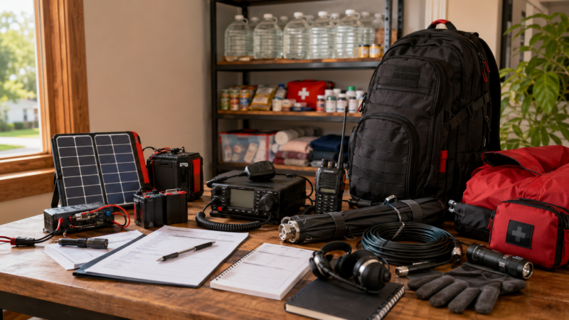
Plan in two layers: a 72-hour communications module and at least two weeks of household readiness. Agency instructions control what deploys. Pack for mobility, weather, medical needs, and safe power—not for an equipment show.
Personal, Safety, and Administration
- Photo ID, license copy, organization credentials, deployment paperwork, and emergency contacts.
- Medicines, glasses or hearing supplies, first aid, water, food, sanitation, clothing, rain gear, gloves, sturdy footwear, and sleep system.
- Required high-visibility garment and PPE; light, cash, notebook, pencils, tape, and ICS/message-log forms.
Radio and Data
- Programmed radio; headset; fuses; adapters; interface cables; feed-line; portable antenna and support; grounding and weather protection.
- Laptop or tablet with current software, charging, offline forms, time synchronization, and tested Winlink configuration—plus paper backup.
- Printed channel plan and contacts; labeled equipment; only authorized frequencies and credentials.
Power
- Charged, known-capacity batteries; fused distribution; standard connectors; meter; chargers; and a plan for charger noise.
- Solar or a power station may extend endurance. Generators require fuel, maintenance, approved outdoor placement, and site permission.
- Load-test the whole station; high-duty-cycle digital transmission drains batteries much faster than receiving.
| Source | Advantages | Limitations | Best preparation step |
|---|---|---|---|
| LiFePO4 battery | Light for usable capacity; stable voltage; many cycles. | Requires compatible charging and cold-weather awareness. | Measure real station runtime and fuse at the battery. |
| Sealed lead-acid | Simple, familiar, and widely available. | Heavy; less usable capacity at high load; shorter cycle life. | Load-test regularly and replace aging batteries. |
| Portable power station | Integrated charging, display, DC and AC outputs. | Inverter noise, proprietary limits, and misleading headline capacity can affect use. | Test receiver noise and runtime before deployment. |
| Solar | Silent renewable charging and useful for extended operations. | Weather, shade, panel angle, and charge-controller noise. | Practice a full charge cycle in realistic conditions. |
| Generator | High continuous output and fast resupply when fuel is available. | Noise, exhaust, fuel logistics, maintenance, and safety controls. | Use only in an approved outdoor location under the site safety plan. |
Earthquake and Ham-Radio Myths
| Myth | Planning fact |
|---|---|
| “A big New Madrid quake will destroy Chicago.” | Chicago is far from the zone. Direct effects are expected to be lower than in southern Illinois, while lifeline, inspection, communications, and mutual-aid consequences may still be significant. |
| “A quiet fault is overdue.” | Earthquakes do not follow a dependable appointment calendar. Probability estimates express uncertainty and do not predict a date. |
| “A handheld radio is an emergency plan.” | A useful operator also needs training, an assignment, antenna and power options, message discipline, logs, and personal sustainment. |
| “Ham Radio takes over when phones fail.” | Emergency managers select the best available path. Amateur Radio supplements authorized systems for specific gaps. |
| “More power is always better.” | Illinois ARES guidance calls for the minimum RF power necessary, conserving energy and reducing interference.[18] |
A SARC Emergency-Preparedness Roadmap
SARC already has the foundation: an EMCOMM committee, repeaters covering much of Chicago’s northwest suburbs, directed weekly nets, and SARC in the Park sessions that test portable stations under non-ideal conditions.[15][24][25] The next step is to connect those activities into a repeatable qualification path.
---
config:
  markdownAutoWrap: true
  flowchart:
    wrappingWidth: 220
    useMaxWidth: true
    nodeSpacing: 40
    rankSpacing: 50
---
flowchart TD
    A["`Join SARC
nets`"]

    B["`Complete ICS-100, ICS-200,
ICS-700, and ICS-800`"]

    C["`Build and test a portable
VHF/UHF station`"]

    D["`Practice directed nets
and ICS-213 traffic`"]

    E["`Configure and exercise
Winlink`"]

    F["`Participate in SARC in the Park
and public-service activities`"]

    G["`Register with local ARES/RACES
or an affiliated agency`"]

    H["`Take part in tabletop, SET,
and earthquake exercises`"]

    I["`Complete an after-action review
and annual requalification`"]

    A --> B
    B --> C
    C --> D
    D --> E
    E --> F
    F --> G
    G --> H
    H --> I
Suggested Annual Club Exercises
| When | Exercise | Measurable objective |
|---|---|---|
| Quarterly | Twenty-minute message-handling drill during or after a regular net. | Pass an ICS-213 without changing names, numbers, priority, or meaning; complete a message log. |
| Spring | Portable-power and simplex coverage day at SARC in the Park. | Operate for four hours without commercial power and document coverage from assigned sites. |
| Summer | Winlink gateway and peer-to-peer exercise. | Send a structured form by two paths and demonstrate offline recovery of the message. |
| Autumn | New Madrid tabletop or Simulated Emergency Test. | Staff net control, EOC, shelter, and field roles through two operational periods with shift relief. |
| Yearly | Served-agency planning meeting and after-action review. | Update contacts, activation method, channel plan, credential requirements, and corrective actions. |
Related SARC Training
- Emergency Communications: committee goals, ICS recommendations, and pathways into ARES, RACES, SATERN, AUXCOMM, and CERT.
- SARC Nets: practice directed-net procedure and maintain operator familiarity.
- SARC Repeaters: verify current frequency, offset, tone, and mode information before every exercise.
- SARC in the Park: test go-boxes, antennas, batteries, and operator workflow away from the home station.
- SARC Calendar: watch for nets, meetings, portable events, and training opportunities.
Call to Action: Train Before the Ground Moves
A New Madrid earthquake is a low-frequency, high-consequence scenario—not a reason for alarm. Build a two-week household plan, secure heavy contents, practice drop-cover-hold, and maintain medicines and family communications. Build radio capability in layers: reliable local operation, portable power, a practiced antenna, formal message skills, Winlink, and ICS familiarity.
SARC members can start by checking into a directed net, operating battery-powered at SARC in the Park, completing core FEMA courses, and joining the next EMCOMM exercise. Those seeking deployment should enroll with the appropriate ARES, RACES, AUXCOMM, CERT, SATERN, or served-agency program.
A disciplined operator who listens, follows direction, sends an exact message, and documents it is more valuable than elaborate untested equipment. SARC’s contribution is a dependable team that is known, trained, safe, and ready to serve.
References
- U.S. Geological Survey, “The New Madrid Seismic Zone,” including science overview and probability FAQ. https://www.usgs.gov/programs/earthquake-hazards/new-madrid-seismic-zone. Accessed July 20, 2026. Return to article.
- Illinois Emergency Management Agency and Office of Homeland Security, Ready Illinois, “Earthquake” and “Two Weeks Ready Campaign.” https://ready.illinois.gov/hazards/earthquake.html. Accessed July 20, 2026. Return to article.
- U.S. Geological Survey, “1811–1812 New Madrid, Missouri Earthquakes.” https://www.usgs.gov/programs/earthquake-hazards/science/1811-1812-new-madrid-missouri-earthquakes. Accessed July 20, 2026. Return to article.
- U.S. Geological Survey, “National Seismic Hazard Model, 2023—Chance of Damaging Earthquake Shaking,” and related 2024 national model release. https://www.usgs.gov/media/images/national-seismic-hazard-model-2023-chance-damaging-earthquake-shaking. Accessed July 20, 2026. Return to article.
- Illinois State Geological Survey, Prairie Research Institute, “Hazards—Earthquakes.” https://isgs.illinois.edu/research/hazards/. Accessed July 20, 2026. Return to article.
- U.S. Geological Survey, McBride and others, “Investigating Possible Earthquake-Related Structure Associated with the November 9, 1968, South-Central Illinois Earthquake.” https://pubs.usgs.gov/publication/70019838. Accessed July 20, 2026. Return to article.
- U.S. Geological Survey, “Catalog of Significant Historical Earthquakes in the Central United States.” https://www.usgs.gov/publications/catalog-significant-historical-earthquakes-central-united-states. Accessed July 20, 2026. Return to article.
- U.S. Geological Survey, “M 5.2—7 km NNE of Bellmont, Illinois,” April 18, 2008 event page. https://earthquake.usgs.gov/earthquakes/eventpage/nm606657. Accessed July 20, 2026. Return to article.
- U.S. Geological Survey, “Map New Madrid Seismic Zone,” public-domain map. https://www.usgs.gov/media/images/map-new-madrid-seismic-zone. Accessed July 20, 2026. Return to article.
- Village of Schaumburg, “Emergency Operations Center.” https://www.villageofschaumburg.com/government/fire/emergency-preparedness/emergency-operations-center. Accessed July 20, 2026. Return to article.
- Cook County, “Emergency Management and Regional Security.” https://www.cookcountyil.gov/agency/emergency-management. Accessed July 20, 2026. Return to article.
- Mutual Aid Box Alarm System—Illinois, “What Is MABAS?” https://www.mabas-il.org/. Accessed July 20, 2026. Return to article.
- Central United States Earthquake Consortium, “New Madrid Seismic Zone Catastrophic Planning Project.” https://cusec.org/new-madrid-seismic-zone/new-madrid-seismic-zone-catastrophic-planning-project/. Accessed July 20, 2026. Return to article.
- ARRL, “Amateur Radio Emergency Service.” https://www.arrl.org/ares. Accessed July 20, 2026. Return to article.
- Schaumburg Amateur Radio Club, “Emergency Communications” and “Emergency Communications Committee.” https://www.n9rjv.org/activities/emergency-communications/ and https://www.n9rjv.org/info/constitution-bylaws/committee-definitions/. Accessed July 20, 2026. Return to article.
- Electronic Code of Federal Regulations, Title 47, Section 97.407, “Radio Amateur Civil Emergency Service.” https://www.ecfr.gov/current/title-47/chapter-I/subchapter-D/part-97/subpart-E/section-97.407. Accessed July 20, 2026. Return to article.
- Cybersecurity and Infrastructure Security Agency, “Communications Unit Training Resources—Auxiliary Communicator.” https://www.cisa.gov/safecom/comu-training-resources. Accessed July 20, 2026. Return to article.
- Illinois ARES, “Emergency Operations All Hazards—ARES/AUXCOMM Incident Operating Practices,” 2026. https://arrl-il.org/ARES/STATE_Combined_Emergency_Operations_All_Hazards.pdf. Accessed July 20, 2026. Return to article.
- Illinois ARES, “Emergency Operations All Hazards,” message-handling and logging provisions, 2026. https://arrl-il.org/ARES/STATE_Combined_Emergency_Operations_All_Hazards.pdf. Accessed July 20, 2026. Return to article.
- Illinois ARES, “Emergency Operations All Hazards,” data communications and Winlink provisions, 2026. https://arrl-il.org/ARES/STATE_Combined_Emergency_Operations_All_Hazards.pdf. Accessed July 20, 2026. Return to article.
- Federal Emergency Management Agency, Emergency Management Institute, “ICS Fillable Forms,” including ICS-213 General Message. https://training.fema.gov/icsresource/icsforms.aspx. Accessed July 20, 2026. Return to article.
- Winlink Global Radio Email, “E-mail With or Without the Internet.” https://winlink.org/content/e_mail_or_without_internet. Accessed July 20, 2026. Return to article.
- Federal Emergency Management Agency, “ICS Form 205—Incident Radio Communications Plan,” version 3.1. https://training.fema.gov/emiweb/is/icsresource/assets/ics%20forms/ics%20form%20205%2C%20incident%20radio%20communications%20plan%20%28v3.1%29.pdf. Accessed July 20, 2026. Return to article.
- Schaumburg Amateur Radio Club, “Repeaters.” https://www.n9rjv.org/repeaters/. Accessed July 20, 2026. Return to article.
- Schaumburg Amateur Radio Club, “Nets” and “SARC in the Park.” https://www.n9rjv.org/info/nets/ and https://www.n9rjv.org/activities/sarc-in-the-park/. Accessed July 20, 2026. Return to article.